{
"cells": [
{
"cell_type": "markdown",
"id": "2ab73f00-58c6-4dbd-8278-284a1577c168",
"metadata": {
"editable": true,
"slideshow": {
"slide_type": "slide"
},
"tags": []
},
"source": [
"# Ultra-long Time Series Forecasting\n",
"\n",
"## Feng Li\n",
"\n",
"### Guanghua School of Management\n",
"### Peking University\n",
"\n",
"\n",
"### [feng.li@gsm.pku.edu.cn](feng.li@gsm.pku.edu.cn)\n",
"### Course home page: [https://feng.li/bdcf](https://feng.li/bdcf)"
]
},
{
"cell_type": "markdown",
"id": "34f1108e-0365-401b-9727-b430a2415a9a",
"metadata": {
"editable": true,
"slideshow": {
"slide_type": "slide"
},
"tags": []
},
"source": [
"## Motivation\n",
"\n",
"- **Ultra-long time series** are increasingly accumulated in many cases.\n",
"\n",
" - hourly electricity demands\n",
" - daily maximum temperatures\n",
" - streaming data generated in real-time\n",
"\n",
"- Forecasting such long time series is **challenging** with traditional approaches.\n",
"\n",
" - time-consuming training process\n",
" - hardware requirements\n",
" - unrealistic assumption about the data generating process\n",
" \n",
"- Some attempts are made in the vast literature.\n",
"\n",
" - discard the earliest observations\n",
" - allow the model itself to evolve over time\n",
" - apply a model-free prediction"
]
},
{
"cell_type": "markdown",
"id": "3cf8b36c-2995-4122-94ac-7eb649b68d43",
"metadata": {
"editable": true,
"slideshow": {
"slide_type": "slide"
},
"tags": []
},
"source": [
"# The Global Energy Forecasting Competition 2017 (GEFCom2017)\n",
"\n",
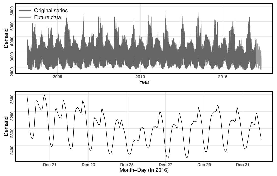
"- Ranging from March 1, 2003 to April 30, 2017 ( $124,171$ time points)\n",
"\n",
"- $10$ hourly electricity load series\n",
"\n",
"- Training periods
March 1, 2003 - December 31, 2016\n",
" \n",
"- Test periods
January 1, 2017 - April 30, 2017
( $h=2,879$ )"
]
},
{
"cell_type": "markdown",
"id": "2936775b-bfc7-4e4b-a268-81308b504e69",
"metadata": {
"editable": true,
"slideshow": {
"slide_type": "slide"
},
"tags": []
},
"source": [
"## An example series from the GEFCom2017 dataset\n",
"\n"
]
},
{
"cell_type": "markdown",
"id": "1d7bf729-de6d-42a1-bdf0-b9cab4f4970f",
"metadata": {
"editable": true,
"slideshow": {
"slide_type": "slide"
},
"tags": []
},
"source": [
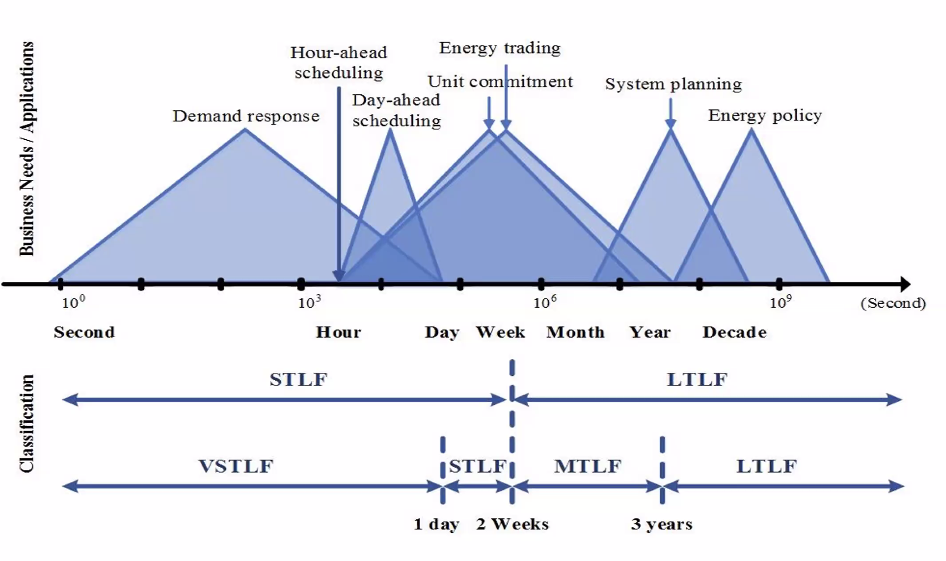
"## Goal of electricity load forecasting\n",
"\n",
"\n"
]
},
{
"cell_type": "markdown",
"id": "e20c69e6-a974-4394-8d35-a69b0b94f98e",
"metadata": {
"editable": true,
"slideshow": {
"slide_type": "slide"
},
"tags": []
},
"source": [
"## Statistical modeling on distributed systems\n",
"\n",
"- Divide-and-conquer strategy\n",
"\n",
"- **Distributed Least Squares Approximation** (DLSA, Zhu, Li & Wang, 2021)\n",
"\n",
" - Solve a large family of regression problems on distributed systems\n",
"\n",
" - Compute local estimators in worker nodes in a parallel manner\n",
"\n",
" - Deliver local estimators to the master node to approximate global estimators by taking a weighted average\n"
]
},
{
"cell_type": "markdown",
"id": "3aada76f-879a-47e7-b56e-c8b5e82c63b8",
"metadata": {
"editable": true,
"slideshow": {
"slide_type": "slide"
},
"tags": []
},
"source": [
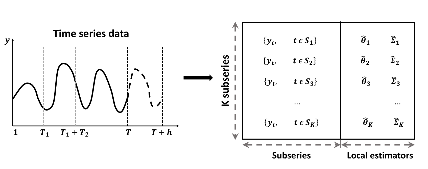
"## Parameter estimation problem\n",
"\n",
"- For an ultra-long time series $\\left\\{y_{t}; t=1, 2, \\ldots , T \\right\\}$. Define $\\mathcal{S}=\\{1, 2, \\cdots, T\\}$ to be the timestamp sequence.\n",
"\n",
"- The parameter estimation problem can be formulated as \n",
"$$\n",
"f\\left( \\theta ,\\Sigma | y_t, t \\in \\mathcal{S} \\right).\n",
"$$\n",
"\n",
"- Suppose the whole time series is split into $K$ subseries with contiguous time intervals, that is $\\mathcal{S}=\\cup_{k=1}^{K} \\mathcal{S}_{k}$.\n",
"\n",
"- The parameter estimation problem is transformed into $K$ **sub-problems** and one **combination problem** as follows:\n",
"$$\n",
"f\\left( \\theta ,\\Sigma | y_t, t \\in \\mathcal{S} \\right) = g\\big( f_1\\left( \\theta_1 ,\\Sigma_1 | y_t, t \\in \\mathcal{S}_1 \\right), \\ldots, f_K\\left( \\theta_K ,\\Sigma_K | y_t, t \\in \\mathcal{S}_K \\right) \\big).\n",
"$$"
]
},
{
"cell_type": "markdown",
"id": "2f4d75fd-ecd6-4170-9d12-fcf0569a99e9",
"metadata": {
"editable": true,
"slideshow": {
"slide_type": "slide"
},
"tags": []
},
"source": [
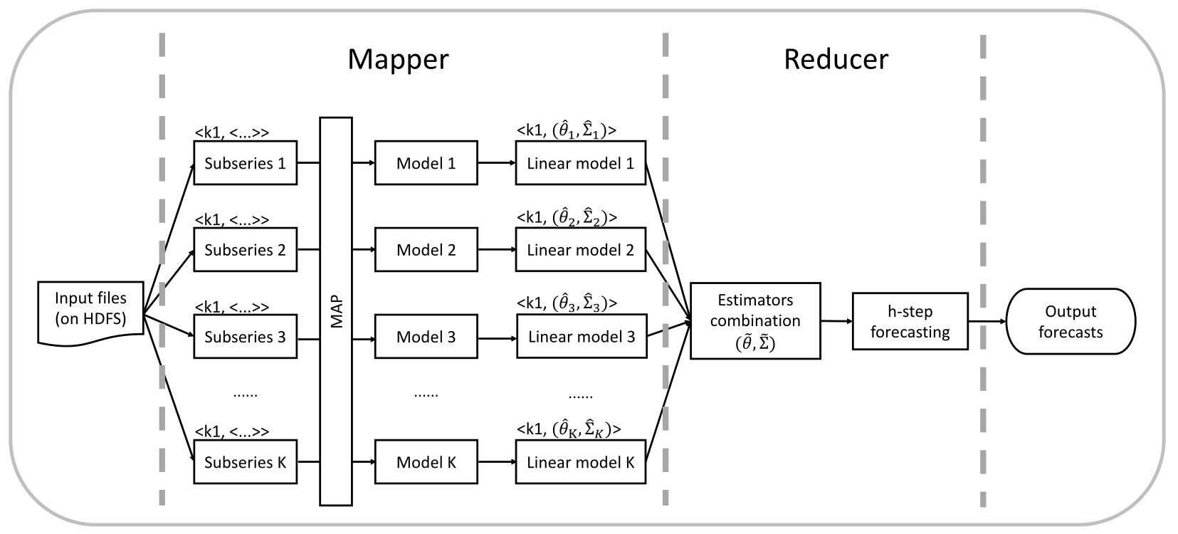
"## Distributed forecasting\n",
"\n",
""
]
},
{
"cell_type": "markdown",
"id": "e1e6b3a6-b303-4e8f-bc68-429471896c08",
"metadata": {
"editable": true,
"slideshow": {
"slide_type": "slide"
},
"tags": []
},
"source": [
"# The proposed framework for time series forecasting on a distributed system\n",
"\n",
"- Step 1: Preprocessing.\n",
"- Step 2: Modeling (assuming that the DGP of subseries remains the same over the short time-windows).\n",
"- Step 3: Linear transformation.\n",
"- Step 4: Estimator combination (minimizing the global loss function).\n",
"- Step 5: Forecasting."
]
},
{
"cell_type": "markdown",
"id": "5a45142e-993e-4331-84cc-85aca10906d4",
"metadata": {
"editable": true,
"slideshow": {
"slide_type": "slide"
},
"tags": []
},
"source": [
""
]
},
{
"cell_type": "markdown",
"id": "6d862092-7b8d-46be-90eb-301daad06389",
"metadata": {
"editable": true,
"slideshow": {
"slide_type": "slide"
},
"tags": []
},
"source": [
"## Why focus on ARIMA models\n",
"\n",
"### Potential\n",
"\n",
"- The most widely used statistical time series forecasting approaches.\n",
"\n",
"- Handle non-stationary series via differencing and seasonal patterns.\n",
"\n",
"- The automatic ARIMA modeling was developed to easily implement the order selection process (Hyndman & Khandakar, 2008).\n",
"\n",
"- Frequently serves asa benchmark method for forecast combinations.\n",
"\n",
"### Limitation\n",
"\n",
"- The likelihood function of such a time series model could hardly scale up."
]
},
{
"cell_type": "markdown",
"id": "7f306875-6a93-4f6f-8c2e-096b321f8b7a",
"metadata": {
"editable": true,
"slideshow": {
"slide_type": "slide"
},
"tags": []
},
"source": [
"# General framework\n",
"- The linear form makes it easy for the estimators combination\n",
"\n",
"- Due to the nature of time dependence, the likelihood function of such time series model could hardly scale up, making it infeasible for massive time series forecasting."
]
},
{
"cell_type": "markdown",
"id": "d2006be5-236a-4ac1-bcc5-71bcf2688a48",
"metadata": {
"editable": true,
"slideshow": {
"slide_type": "slide"
},
"tags": []
},
"source": [
"## Automatic ARIMA modeling\n",
"\n",
"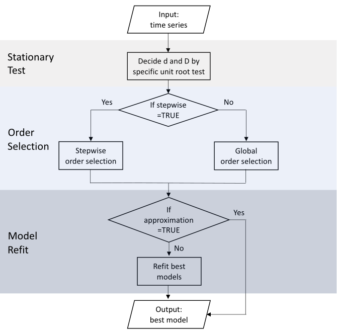"
]
},
{
"cell_type": "markdown",
"id": "d0c60116-fc31-4c1f-8bd5-5a5dc9406d8f",
"metadata": {
"editable": true,
"slideshow": {
"slide_type": "slide"
},
"tags": []
},
"source": [
"## Necessity of linear transformation\n",
"\n",
"- Condition of distributed forecasting\n",
"\n",
"- Local models fitted on the subseries are capable of being combined to result in the global model for the whole series.\n",
"\n",
"- A seasonal ARIMA model is generally defined as\n",
"\\begin{align}\n",
"\\left(1-\\sum_{i=1}^{p}\\phi_{i} B^{i}\\right) \\left(1-\\sum_{i=1}^{P}\\Phi_{i} B^{im}\\right)(1-B)^{d}\\left(1-B^{m}\\right)^{D} \\left(y_{t} - \\mu_0 - \\mu_1 t \\right) \\nonumber \\\\\n",
"=\\left(1+\\sum_{i=1}^{q}\\theta_{i} B^{i}\\right)\\left(1+\\sum_{i=1}^{Q}\\Theta_{i} B^{im}\\right) \\varepsilon_{t}.\n",
"\\end{align}\n",
"\n",
"- Properties of ARMA models: stationarity, causality, and invertibility.\n",
" \n",
"- A causal invertible model should have all the roots outside the unit circle.\n",
" \n",
"- Directly combining ARIMA models would lead to a global ARIMA model with roots inside the unit circle.\n",
"\n",
"- The directly combined ARIMA models will be ill-behaved, thus resulting in numerically unstable forecasts.\n",
"\n"
]
},
{
"cell_type": "markdown",
"id": "8f425dd4-9902-48b1-8076-0d63459fa460",
"metadata": {
"editable": true,
"slideshow": {
"slide_type": "slide"
},
"tags": []
},
"source": [
"## Linear representation\n",
"\n",
"\n",
"- The **linear representation** of the original seasonal ARIMA model can be given by\n",
"\\begin{equation}\n",
"y_t = \\beta_0 + \\beta_1 t + \\sum_{i=1}^{\\infty}\\pi_{i}y_{t-i} + \\varepsilon_{t},\n",
"\\end{equation}\n",
"where \n",
"\\begin{equation}\n",
"\\beta_0 = \\mu_0 \\left( 1- \\sum_{i=1}^{\\infty}\\pi_{i} \\right) + \\mu_1 \\sum_{i=1}^{\\infty}i\\pi_{i} \n",
"\\qquad \\text{and}\\qquad \n",
"\\beta_1 = \\mu_1 \\left( 1- \\sum_{i=1}^{\\infty}\\pi_{i} \\right).\n",
"\\end{equation}\n",
"\n",
"- This can be extended easily to involve covariates.\n",
"\n",
"- For a general seasonal ARIMA model, by using multiplication and long division of polynomials, we can obtain the final converted linear representation in this form.\n",
"- In this way, all ARIMA models fitted for subseries can be converted into this linear form.\n"
]
},
{
"cell_type": "markdown",
"id": "65263f62-892e-4cb2-933a-e84524d44bac",
"metadata": {
"editable": true,
"slideshow": {
"slide_type": "slide"
},
"tags": []
},
"source": [
"## Estimators combination\n",
"\n",
"- Some excellent statistical properties of the global estimator obtained by DLSA has been proved (Zhu, Li & Wang 2021, JCGS).\n",
"\n",
"- We extend the DLSA method to solve time series modeling problem.\n",
"\n",
"- Define $\\mathcal{L}(\\theta; y_t)$ to be a second order differentiable loss function, we have\n",
"\\begin{align}\n",
"\\label{eq:loss}\n",
"\\mathcal{L}(\\theta) &=\\frac{1}{T} \\sum_{k=1}^{K} \\sum_{t \\in \\mathcal{S}_{k}} \\mathcal{L}\\left(\\theta ; y_{t}\\right) \\nonumber \\\\\n",
"&=\\frac{1}{T} \\sum_{k=1}^{K} \\sum_{t \\in \\mathcal{S}_{k}}\\left\\{\\mathcal{L}\\left(\\theta ; y_{t}\\right)-\\mathcal{L}\\left(\\hat{\\theta}_{k} ; y_{t}\\right)\\right\\}+c_{1} \\nonumber \\\\ \n",
"& \\approx \\frac{1}{T} \\sum_{k=1}^{K} \\sum_{t \\in \\mathcal{S}_{k}}\\left(\\theta-\\widehat{\\theta}_{k}\\right)^{\\top} \\ddot{\\mathcal{L}}\\left(\\hat{\\theta}_{k} ; y_{t}\\right)\\left(\\theta-\\hat{\\theta}_{k}\\right)+c_{2} \\nonumber \\\\\n",
"&\\approx \\sum_{k=1}^{K} \\left(\\theta-\\hat{\\theta}_{k}\\right)^{\\top} \\left(\\frac{T_k}{T} \\widehat{\\Sigma}_{k}^{-1}\\right) \\left(\\theta-\\hat{\\theta}_{k}\\right)+c_{2}.\n",
"\\end{align}\n",
"\n",
"- The next stage entails solving the problem of combining the local \n",
"-\tTaylor’s theorem & the relationship between the Hessian and covariance matrix for Gaussian random variables\n",
"-\tThis leads to a weighted least squares form\n"
]
},
{
"cell_type": "markdown",
"id": "8dbc31bd-3fc3-43ab-a0c3-1ef1d5634dca",
"metadata": {
"editable": true,
"slideshow": {
"slide_type": "slide"
},
"tags": []
},
"source": [
"## Estimators combination\n",
"\n",
"- The **global estimator** calculated by minimizing the weighted least squares takes the following form\n",
"\\begin{align}\n",
"\\tilde{\\theta} &= \\left(\\sum_{k=1}^{K}\\frac{T_k}{T}\\widehat{\\Sigma}_{k}^{-1}\\right)^{-1}\\left(\\sum_{k=1}^{K}\\frac{T_k}{T}\\widehat{\\Sigma}_{k}^{-1}\\hat{\\theta}_{k}\\right), \\\\\n",
"\\tilde{\\Sigma} &= \\left(\\sum_{k=1}^{K}\\frac{T_k}{T}\\widehat{\\Sigma}_{k}^{-1}\\right)^{-1}.\n",
"\\end{align}\n",
"\n",
"- $\\widehat{\\Sigma}_{k}$ is not known and has to be estimated.\n",
"\n",
"- We approximate a GLS estimator by an OLS estimator (e.g., Hyndman et al., 2011) while still obtaining consistency.\n",
"\n",
"- We consider approximating $\\widehat{\\Sigma}_{k}$ by $\\hat{\\sigma}_{k}^{2}I$ for each subseries.\n",
"\n",
" - simplify the computations\n",
" - reduce the communication costs in distributed systems.\n",
"\n",
"- The global estimator and its covariance matrix can be obtained.\n",
"- The covariance matrix of subseries is not known, so we estimate it by $\\sigma^2\\times I$."
]
},
{
"cell_type": "markdown",
"id": "5e3b7345-33a6-47c6-ae5d-6d779c82934d",
"metadata": {
"editable": true,
"slideshow": {
"slide_type": "slide"
},
"tags": []
},
"source": [
"## Output forecasts\n",
"\n",
"- The $h$-step-ahead point forecast can be calculated as\n",
"\\begin{equation}\n",
"\\hat{y}_{T+h | T}=\\tilde{\\beta}_{0}+\\tilde{\\beta}_{1}(T+h)+\\left\\{\\begin{array}{ll}\\sum_{i=1}^{p} \\tilde{\\pi}_{i} y_{T+1-i}, & h=1 \\\\ \\sum_{i=1}^{h-1} \\tilde{\\pi}_{i} \\hat{y}_{T+h-i | T}+\\sum_{i=h}^{p} \\tilde{\\pi}_{i} y_{T+h-i}, & 1 1 \\\\\n",
"\\end{array},\n",
"\\right.\n",
"\\end{equation}\n",
" where $\\tilde{\\sigma}^{2}= \\operatorname{tr}(\\tilde{\\Sigma})/p$.\n"
]
},
{
"cell_type": "markdown",
"id": "decf67e4-8df9-4136-b2d1-377b10637ded",
"metadata": {
"editable": true,
"slideshow": {
"slide_type": "slide"
},
"tags": []
},
"source": [
"# Conclusions\n",
"\n",
"- We propose a **distributed time series forecasting framework** using the industry-standard MapReduce framework.\n",
"\n",
"- The local estimators trained on each subseries are combined using **weighted least squares** with the objective of minimizing a global loss function.\n",
"\n",
"- Our framework\n",
"\n",
" - works better than competing methods for **long-term forecasting**.\n",
" \n",
" - achieves improved **computational efficiency** in optimizing the model parameters.\n",
" \n",
" - allows that the **DGP** of each subseries could vary.\n",
" \n",
" - can be viewed as a **model combination** approach."
]
}
],
"metadata": {
"kernelspec": {
"display_name": "Python3.12 (PySpark3.5.4)",
"language": "python",
"name": "pyspark"
},
"language_info": {
"codemirror_mode": {
"name": "ipython",
"version": 3
},
"file_extension": ".py",
"mimetype": "text/x-python",
"name": "python",
"nbconvert_exporter": "python",
"pygments_lexer": "ipython3",
"version": "3.12.8"
}
},
"nbformat": 4,
"nbformat_minor": 5
}